
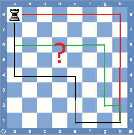
A rook is placed in the corner of a standard (8 x 8) chessboard. Every minute, it makes a legal move, where each move has the same probability of being chosen. What is the expected number of minutes for the rook to reach the opposite corner?
This puzzle was proposed at the HMMT November 2015 competition (Theme round, problem #8). HMMT is the Harvard-MIT Mathematics Tournament, one of the largest and most prestigious high school competitions in the world. Each event gathers close to 1,000 students from around the globe, including top scorers at both U.S. and international math olympiads.
The minimum number of moves (and minutes) for the rook, being at one corner, to get to the opposite one is just 2 (two); the probability that this happens is 1/7 * 1/14 + 1/7 * 1/14 = 1/49 (almost 2%). On the other hand, the set (or more exactly, the tree) of possible “journeys” for the rook, which account for the remaining 98%, is infinite; each journey takes more (or much more) than two minutes. What would be the expected number of minutes for the rook to get to its final destination: ten, twenty, fifty? One hundred maybe?
Simulation
One obvious solution is to simulate a “reasonable” number (say 1 million times) of random rook journeys, each one starting at the same corner square and ending on the opposite one. The C program below took roughly 1.3 seconds on my PC to print the average journey duration: 70.022925 minutes.
#include <time>
#include
#include
typedef struct {
int x;
int y;
}
square;
square rookMove(square sq) {
int newCoord = (rand() % 8) + 1;
if (rand() % 2) {
while (newCoord == sq.x)
newCoord = (rand() % 8) + 1;
sq.x = newCoord;
} else {
while (newCoord == sq.y)
newCoord = (rand() % 8) + 1;
sq.y = newCoord;
}
return sq;
}
float rookJourneys(int trials) {
int moves = 0;
for (int i = 0; i < trials; i++) {
square sq = {
1,
1
};
while (sq.x != 8 || sq.y != 8) {
sq = rookMove(sq);
moves++;
}
}
return (float) moves / (float) trials;
}
void main() {
srand(time(NULL));
printf("%.6f\n", rookJourneys(1000000));
}
Markov chain
We can also attack this problem treating the sequence of rook moves as a discrete-time Markov chain.
A Markov chain (or process) can be described by a set of states, 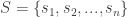


The probabilities 
Let’s now see the what are the particular characteristics of our newly discovered Markov chain. One can associate a unique state to each of the 64 squares the rook can eventually go. The rook initial square — which coordinates are (1, 1) — is the starting state for all sequences. It’s also easy to see that all transition probabilities of the form 
Our Markov chain has another interesting property: it has an absorbing state — with coordinates (8,8) — a state it is impossible to leave, meaning that 


The Magma script (see box below) calculates the expected number of minutes taken by the rook to get to the final square starting on any other square. It follows the very clear and interesting explanation about absorbing Markov chains found in “Introduction to Probability“, Gristead & Snell (see chap. 11, section 11.2, pp. 416-419).
/**
* Square (i, j) on the board (1 <= i,j <= 8) is unequivocally
* represented by state (i, j) = 8 * (i - 1) + (j - 1) + 1.
* Note that 1 <= state (i, j) <= 64.
*/
function state (i, j)
return 8 * (i - 1) + (j - 1) + 1;
end function;
/**
* This function returns a SeqEnum containing the coordinates
* (row/column) associated with the input state (1 <= i,j <= 8).
*/
function unstate (n)
return [(n - 1) mod 8 + 1, (n - 1) div 8 + 1];
end function;
/**
* Entry Q[u, v] on the transition probability matrix below
* denotes the probability of a transition from transient
* state u to transient state v.
*/
Q := ZeroMatrix (RealField (), 63, 63);
for i, j, k in [1 .. 8] do
// make sure the absorbing state (8, 8) is excluded
if i + j ne 16 and i + k ne 16 and j + k ne 16 then
if k ne j then
// probability to move on the same row: 1/2
// probability to move to a square on that row: 1/7
Q [state (i, j)][state (i, k)] := (1 / 2) * (1 / 7);
end if;
if k ne i then
// probability to move on the same column: 1/2
// probability to move to a square on that column: 1/7
Q [state (i, j)][state (k, j)] := (1 / 2) * (1 / 7);
end if;
end if;
end for;
/**
* N is the 'fundamental matrix' for P, the transition probability
* matrix for all allowed states, either transient or absorbing.
*/
I := IdentityMatrix (RealField (), 63);
N := (I - Q) ^ -1;
c := Matrix (RealField (), 63, 1, [1.0 : k in [1 .. 63]]);
t := N * c;
printf "Starting square\t Expected time to reach destination\n";
for n in [1 .. 63] do
printf "    (%o, %o)\t t = %o\n",
unstate(n)[1], unstate(n)[2], t[n][1];
end for;
In simple terms, this script evaluates the expression below for each one of the 63 possible starting squares:
![E_{ij} = \displaystyle\sum_{\substack{all \, paths\\ starting \, on\\ square \, (i,j)}}^{} probability \, [path] \, \times \, time \, (path)](https://s0.wp.com/latex.php?latex=E_%7Bij%7D+%3D+%5Cdisplaystyle%5Csum_%7B%5Csubstack%7Ball+%5C%2C+paths%5C%5C+starting+%5C%2C+on%5C%5C+square+%5C%2C+%28i%2Cj%29%7D%7D%5E%7B%7D%C2%A0probability+%5C%2C+%5Bpath%5D+%5C%2C+%5Ctimes+%5C%2C+time+%5C%2C+%28path%29&bg=ffffff&fg=333333&s=0&c=20201002)
Magma is a commercial software package designed for computations in algebra, number theory, algebraic geometry and algebraic combinatorics. The mentioned script was executed using Magma Calculator, a web interface that provides free access to the Magma software under certain run time and script size restrictions.
After just 0.3 seconds, we have the desired results (see box below). It seems that the expected times could probably be integers (63 and 70), something we haven’t been able to notice during the simulation session.
Using the same tool, it’s also easy to evaluate the probability that the rook takes, say, 500 minutes, to reach the destination square starting from the square (1, 1). All that is needed is to execute the command ((Q^500)*c [state(1, 1)], which gives 0.066% as the answer.
Starting square  Expected time to reach destination
(1, 1)       t = 70.0000000000000000000000000016
(2, 1)       t = 70.0000000000000000000000000030
(3, 1)       t = 70.0000000000000000000000000030
(4, 1)       t = 70.0000000000000000000000000027
(5, 1)       t = 70.0000000000000000000000000025
(6, 1)       t = 70.0000000000000000000000000030
(7, 1)       t = 70.0000000000000000000000000024
(8, 1)       t = 63.0000000000000000000000000025
(1, 2)       t = 70.0000000000000000000000000023
(2, 2)       t = 70.0000000000000000000000000019
...                         ...
(6, 7)       t = 70.0000000000000000000000000025
(7, 7)       t = 70.0000000000000000000000000021
(8, 7)       t = 63.0000000000000000000000000017
(1, 8)       t = 63.0000000000000000000000000018
(2, 8)       t = 63.0000000000000000000000000026
(3, 8)       t = 63.0000000000000000000000000022
(4, 8)       t = 63.0000000000000000000000000023
(5, 8)       t = 63.0000000000000000000000000023
(6, 8)       t = 63.0000000000000000000000000027
(7, 8)       t = 63.0000000000000000000000000023
Conditional probabilities
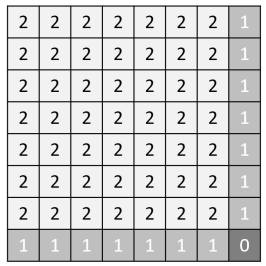
One can further improve the Markovian approach used by looking at the pattern showed in the previous results. Considering the minimum number of moves taken by the rook to get to the destination square, one can divide the chessboard squares into just three types, thus greatly reducing the size of the transition probabilities matrix from 64×64 to only 3×3.
For the sake of notation, we call a type n square any one from which the rook must take at least n move(s), or second(s), to get to the target square. This way, the chessboard can be partitioned into 1 (one) destination square (type 0), 14 (fourteen) “edge” squares (type 1) and 49 (forty-nine) remaining squares (type 2). For all type 1 squares, the expected time is close to 63 minutes while for every type 2 one the expected time is a little bit longer, around 70 minutes.
A much simpler transition probability matrix can then be defined taking into account only five transitions: 


![p \, [type \, i \rightarrow type \, j]](https://s0.wp.com/latex.php?latex=p+%5C%2C+%5Btype+%5C%2C+i+%5Crightarrow+type+%5C%2C+j%5D&bg=ffffff&fg=333333&s=0&c=20201002)
Let the expected number of minutes it will take the rook to reach the destination square from any 


The transition probabilites are easy to calculate:


(of course, 
We can now solve the equation system, which gives the solution
This approach not only is simple but also powerful since it definitely shows that the expected time is an integer. It can also be easily extended to chessboards of other sizes, e.g. 10×10 or 15×15.
